PRUNING BY ACTIVE ATTENTION MANIPULATION Zahra Babaiee Computer Science Department

2025-05-02 0 0 773.71KB 16 页 10玖币

侵权投诉

PRUNING BY ACTIVE ATTENTION MANIPULATION

Zahra Babaiee

Computer Science Department

Technical University of Vienna

zahra.babiee@tuwien.ac.at

Lucas Liebenwein

EE and CS Department

MIT

lucas@mit.edu

Ramin Hasani

EE and CS Department

MIT

rhasani@mit.edu

Daniela Rus

EE and CS Department

MIT

rus@mit.edu

Radu Grosu

Computer Science Department

Technical University of Vienna

radu.grosu@tuwien.ac.at

ABSTRACT

Filter pruning of a CNN is typically achieved by applying discrete masks on the

CNN’s ﬁlter weights or activation maps, post-training. Here, we present a new

ﬁlter-importance-scoring concept named pruning by active attention manipulation

(PAAM), that sparsiﬁes the CNN’s set of ﬁlters through a particular attention

mechanism, during-training. PAAM learns analog ﬁlter scores from the ﬁlter

weights by optimizing a cost function regularized by an additive term in the scores.

As the ﬁlters are not independent, we use attention to dynamically learn their

correlations. Moreover, by training the pruning scores of all layers simultaneously,

PAAM can account for layer inter-dependencies, which is essential to ﬁnding

a performant sparse sub-network. PAAM can also train and generate a pruned

network from scratch in a straightforward, one-stage training process without

requiring a pre-trained network. Finally, PAAM does not need layer-speciﬁc

hyperparameters and pre-deﬁned layer budgets, since it can implicitly determine

the appropriate number of ﬁlters in each layer. Our experimental results on different

network architectures suggest that PAAM outperforms state-of-the-art structured-

pruning methods (SOTA). On CIFAR-10 dataset, without requiring a pre-trained

baseline network, we obtain 1.02% and 1.19% accuracy gain and 52.3% and 54%

parameters reduction, on ResNet56 and ResNet110, respectively. Similarly, on

the ImageNet dataset, PAAM achieves

1.06%

accuracy gain while pruning

51.1%

of the parameters on ResNet50. For Cifar-10, this is better than the SOTA with a

margin of 9.5% and 6.6%, respectively, and on ImageNet with a margin of 11%.

1 INTRODUCTION

End

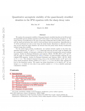
loss

epoch

Warm-up on dense network Train

Train sparse-network’s weights Fine-tune sparse network

PAAM

Pruning by Active Attention Manipulation (PAAM)

Figure 1: Sensitivity-based ﬁlter pruning schedule.

Convolutional Neural Networks (CNNs) LeCun

et al. (1989) are used nowadays in a wide variety

of computer-vision tasks. Large CNNs in par-

ticular, achieve considerable performance levels,

but with signiﬁcant computation, memory, and

energy footprints, respectively Sui et al. (2021).

As a consequence, they cannot be effectively em-

ployed in resource-limited environments such

as mobile or embedded devices. It is therefore

essential to create smaller models, that can per-

form well without signiﬁcantly sacriﬁcing their

accuracy and performance. This goal can be accomplished by either designing smaller, but performant,

network architectures Lechner et al. (2020); Tan & Le (2019) or by ﬁrst training an over-parameterized

network, and sparsifying it thereafter, by pruning its redundant parameters Han et al. (2016); Lieben-

wein et al. (2020; 2021). Neural-network pruning is deﬁned as systematically removing parameters

from an existing neural network Hoeﬂer et al. (2021). It is a popular technique to reduce growing

arXiv:2210.11114v1 [cs.CV] 20 Oct 2022

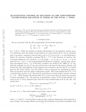
Figure 2: PAAM learns the importance scores of the ﬁlters from the ﬁlter weights.

energy and performance costs and to support deployment in resource-constrained environments such

as smart devices. Various pruning approaches have been developed, and this has gained considerable

attention over the past few years Zhu & Gupta (2017); Sui et al. (2021); Liebenwein et al. (2021);

Peste et al. (2021); Frantar et al. (2021); Deng et al. (2020).

Pruning methods are categorized into either unstructured or structured. The ﬁrst, remove individual

weight-parameters, only Han et al. (2016). The second, remove entire groups, by pruning neurons,

ﬁlters, or channels, respectively Anwar et al. (2017); Li et al. (2019); He et al. (2018b); Liebenwein

et al. (2020). As modern hardware is tuned towards dense computations, structured pruning offers a

more favorable balance between accuracy and performance Hoeﬂer et al. (2021). A very prominent

family of structured-pruning methods is ﬁlter pruning. Choosing which ﬁlters to remove according to

a carefully chosen importance metric (or ﬁlter score) is an essential part of any method in this family.

Data-free methods solely rely on the value of weights, or the network structure, in order to determine

the importance of ﬁlters. Magnitude pruning, for example, is one of the simplest and most common of

such methods. It prunes the ﬁlters that have the smallest weight-values in the

norm. Data-informed

methods focus on the feature maps generated from the training data (or a subset of samples) rather

than the ﬁlters alone. These methods vary from sensitivity-based approaches (which consider the

statistical sensitivity of the output feature maps with regard to the input data Malik & Naumann

(2020); Liebenwein et al. (2020)), to correlation-based methods (with an inter-channel perspective, to

keep the least similar (or least correlated) feature maps Sun et al. (2015); Sui et al. (2021)).

Both data-free and data-informed methods generally determine the importance of a ﬁlter in a given

layer, locally. However, ﬁlter-importance is a global property, as it changes relative to the selection of

the ﬁlters in the previous and next layers. Moreover, determining the optimal ﬁlter-budget for each

layer (a vital element of any pruning method), is also a challenge, that all local, importance-metric

methods face. The most trivial way to overcome these challenges, is to evaluate the network loss

with and without each combination of

candidate ﬁlters out of

. However, this approach would

require the evaluation of N

ksubnetworks, which is in practice impossible to achieve.

Training-aware pruning methods aim to learn binary masks for turning on and off each ﬁlter. A

regularization metric often accompanies them, with a penalty guiding the masks to the desired

budget. Mask learning, simultaneously for all ﬁlters, is an effective method for identifying a globally

optimal subset of the network. However, due to the discrete nature of the ﬁlters and binary masks,

the optimization problem is generally non-convex and NP-hard. A simple trick of many recent

works Gao et al. (2020; 2021); Li et al. (2022) is to use straight-through estimators Bengio et al.

(2013) to calculate the derivatives, by considering binary functions as identities. While ingenious,

this precludes learning the relative importance of ﬁlters among each other. Even more importantly,

the on-off bits within the masks are assumed to be independent, which is a gross oversimpliﬁcation.

This paper solves the above problems by introducing PAAM, a novel end-to-end pruning method, by

active attention manipulation. PAAM also employs an

regularization technique, encouraging ﬁlter-

score decrease. However, PAAM scores are analog, and multiply the activation maps during score

training. Moreover, a proper score spread is ensured through a specialized activation function. This

allows PAAM to learn the relative importance of ﬁlters globally, through gradient descent. Moreover,

the scores are not considered independent, and their hidden correlations are learned in a scalable

fashion, by employing an attention mechanism speciﬁcally tuned for ﬁlter scores. Given a global

pruning budget, PAAM ﬁnds the optimal pruning threshold from the cumulative histogram of ﬁlter

scores, and keeps only the ﬁlters within the budget. This relieves PAAM from having to determine

per layer allocation budgets in advance. PAAM then retrains the network without considering the

scores. This process is repeated until convergence. PAAM pipeline is shown in Figures 1-2. Our

experimental results show that PAAM yields higher pruning ratios while preserving higher accuracy.

In summary, this work has the following contributions:

We introduce PAAM, an end-to-end algorithm that learns the importance scores directly

from the network weights and ﬁlters. Our method allows extracting hidden correlations in

the ﬁlter weights for training the scores, rather than relying only on the weight magnitudes.

The feature maps are multiplied by our learned scores during training. This way our method

implicitly accounts for the data samples through loss propagation, enabling PAAM to enjoy

the advantages of both data-free and data-informed methods.

PAAM automatically calculates global importance scores for all ﬁlters and determines

layer-speciﬁc budgets with only one global hyper-parameter.

We empirically investigate the pruning performance of PAAM in various pruning tasks

and compare it to advanced state-of-the-art pruning algorithms. Our method proves to be

competitive and yields higher pruning ratios while preserving higher accuracy.

2 PRUNING BY ACTIVE ATTENTION MANIPULATION ALGORITHM

In this section, we ﬁrst introduce our notation and then incrementally describe our pruning algorithm.

2.1 Notation.

The ﬁlter weights of layer

are given by the tuple

Fl∈IRF×C×K×K

where

is the

number of ﬁlters,

the number of input channels, and

the size of the convolutional kernel. The

feature maps of layer

are given by the tuple

Al∈IRF×H×W

where

and

are the image height

and width respectively. For simplicity, we ignore the batch dimension in our formulas.

2.2 Score Learning.

The score-learning function of PAAM, for a layer

of the CNN to be pruned,

can be intuitively understood as a single-layer independent network, whose inputs are the ﬁlter

weights

of layer

, and the outputs are the scores

associated to the ﬁlters. The network ﬁrst

transforms the input weights

to a score vector

FlWF

, whose length equals the number

ﬁlters of layer

, and then passes the result through an activation function

, properly spreading the

scores within the

[0,1 + ]

interval. The resulting scores are then used by an

regularization term of

the cost function. The choice of

and regularization term is discussed in the next sections. Formally:

Sl=φ(FlWF)(1)

where

is the activation function and

WF∈IR(F×C×K×K)×F

is the weight matrix. This transfor-

mation, through

and

(vanilla PAM), is similar to additive attention Bahdanau et al. (2014).

We will therefore refer in the following to the score-learning network as the attention network (AN).

Intuitively, the AN weight matrix

captures the hidden correlations among ﬁlters. Unfortunately,

for layers with a large number of ﬁlters, as for ImageNet, this matrix will become too large to train.

To capture the correlations in a scalable fashion, we would like to ﬁrst partition the input in chunks,

compute the correlations within each chunk, and then compute the correlations among chunks. But

this is exactly what a scaled dot-product attention achieves Vaswani et al. (2017a). First, PAAM

reformats the input as a binary matrix

Fl∈IR(F)×(C×K×K)

, where the chunks are its rows. Second,

it obtains the correlations within each chunk as the queries

Ql=FlWQ

and keys

Kl=FlWK

. Here,

the query and key weight matrices

WQ, W K∈IR(C×K×K)×dl

are much smaller, as they consider

only a chunk, and

dl=F

is the hidden dimension of the layer. The queries and keys are of shape

Ql, Kl∈IR(F)×(dl)

. Third, PAAM obtains the cross correlations among chunks by multiplying

the query matrix

with the transpose

of the key matrix. Finally, the scores are obtained by

averaging and normalizing the result, and passing it through the activation function φ. Formally:

Sl=φ(mean(Ql×KT

α√dl

)(2)

where

is a scaling factor that we tune. Note that PAAM does not need to learn the value-weight

matrix, compute the values, and multiply them with the above result, as it is only interested in the

correlation among ﬁlters. Learning ﬁlter weights is left to CNN training. However, the scores

learned by PAAM, are then pointwise () multiplied by the feature maps Alof the same layer:

l=SlAl(3)

The closer a ﬁlter score is to

, the more the corresponding feature map is preserved. Note also that

by using an analog value for scores while training the AN, allows PAAM to compare the relative

importance of scores later on. In particular, this is useful when PAAM employs the globally allocated

budget, and the cumulative score distribution, to select the ﬁlters to be used during CNN training.

2.3 Activation Function.

SoftMax is the typical choice of activation function in additive attention

when computing importance Vaswani et al. (2017b). However, SoftMax is not a suitable choice for

ﬁlter scores. While the range of its outputs is between

and

, the sum of its outputs has to be

meaning that either all scores will have a small value, or there will be only one score with value 1.

In contrast to SoftMax, we would intuitively want that many ﬁlter scores are possibly close to

More formally, the scores should have the following three main attributes: 1) All ﬁlter scores should

have a positive value that ranges between

and

, as is the case in SoftMax. 2) All ﬁlter scores should

adapt from their initial value of

, as we start with a completely dense model. 3) The ﬁlter-scores

activation function should have non-zero gradients over their entire input domain.

Figure 3: The leaky-exponen-

tial activation function.

Sigmoidal activations satisfy Attributes

and

. However, they have

difﬁculties with Attribute

. For high temperatures, sigmoids behave

like steps, and scores quickly converge to

. The chance these

scores change again is very low, as the gradient is close to zero at

this point. Conversely, for low temperatures, scores have a hard

time converging to

. Finding the optimal temperature needs an

extensive search for each of the layers separately. Finally, starting

from a dense network with all scores set to 1is not feasible.

To satisfy Attributes

, we designed our own activation function,

as shown in Figure 3. First, in order to ensure that scores are positive,

we use an exponential activation function and learn its logarithm

value. Second, we allow the activation to be leaky, by not saturating it at

, as this would result in

gradients, and scores getting stuck at

. Formally, our leaky-exponential activation function is deﬁned

as follows, where ais a small value (an ablation study in provided in Appendix):

φ(x) = exif x < 0

1.0 + ax if x≥0(4)

2.4 Optimization Problem.

The PAAM optimization problem can be formulated as in Equation (5),

where

is the CNN loss function, and

is the CNN function with inputs

, labels

, and parameters

, modulated by the AN with inputs the ﬁlter weights, parameters

, and outputs the scores

. Let

kg(Sl, p)k1

denote the

-norm of the binarized ﬁlter scores of layer

the number of ﬁlters of

layer

the number of layers, and

the pruning ratio. Then PAAM should preserve only as many

ﬁlters as desired by p, while minimizing at the same time the loss function.

min

VL(y, f(x;W, S)) s.t.

l=0 kg(Sl, p)k1−p

l=0

Fl= 0 (5)

Function

g(Sl, p)

is discussed in next section. The budget constraint is addressed by adding an

regularization term to the loss function, while training the weights of the AN. This term employs the

analog scores of the ﬁlters in each layer, which are computed as described above. Formally:

L0(S) = L(y, f(x;W, S)) + λ

l=0 kSlk1(6)

where

is a global hyper-parameter controlling the regularizer’s effect on the total loss. Since the

loss function consists now of both classiﬁcation accuracy and the

-norm cost of the scores, reducing

ﬁlter scores to decrease l1cost, directly inﬂuences accuracy as scores multiply the activation maps.

In more detail, by incorporating the classiﬁcation and the

-norm of the scores in the loss function,

the effect of the score of each ﬁlter is accounted for in the loss value in two ways:

文档加载中……请稍候！
如果长时间未打开，您也可以点击刷新试试。

下载文档到电脑，查找使用更方便

10 玖币 0人已下载

立即下载

摘要：

PRUNINGBYACTIVEATTENTIONMANIPULATIONZahraBabaieeComputerScienceDepartmentTechnicalUniversityofViennazahra.babiee@tuwien.ac.atLucasLiebenweinEEandCSDepartmentMITlucas@mit.eduRaminHasaniEEandCSDepartmentMITrhasani@mit.eduDanielaRusEEandCSDepartmentMITrus@mit.eduRaduGrosuComputerScienceDepartmentTechni...

展开>> 收起<<

PRUNING BY ACTIVE ATTENTION MANIPULATION Zahra Babaiee Computer Science Department.pdf

共16页,预览4页

还剩页未读，继续阅读

声明：本站为文档C2C交易模式，即用户上传的文档直接被用户下载，本站只是中间服务平台，本站所有文档下载所得的收益归上传人(含作者)所有。玖贝云文库仅提供信息存储空间，仅对用户上传内容的表现方式做保护处理，对上载内容本身不做任何修改或编辑。若文档所含内容侵犯了您的版权或隐私，请立即通知玖贝云文库，我们立即给予删除！

PRUNING BY ACTIVE ATTENTION MANIPULATION Zahra Babaiee Computer Science Department

相关推荐

开通VIP享超值会员特权

作者详情

相关内容

热门标签

举报选择: