Fast gradient estimation for variational quantum algorithms

2025-04-26 0 0 1.28MB 26 页 10玖币

侵权投诉

Lennart Bittel, Jens Watty, and Martin Kliesch

Institute for Theoretical Physics, Heinrich Heine University Düsseldorf, Germany

Many optimization methods for training

variational quantum algorithms are based on

estimating gradients of the cost function. Due

to the statistical nature of quantum measure-

ments, this estimation requires many circuit

evaluations, which is a crucial bottleneck of the

whole approach. We propose a new gradient

estimation method to mitigate this measure-

ment challenge and reduce the required mea-

surement rounds. Within a Bayesian frame-

work and based on the generalized parame-

ter shift rule, we use prior information about

the circuit to ﬁnd an estimation strategy that

minimizes expected statistical and systematic

errors simultaneously. We demonstrate that

this approach can signiﬁcantly outperform tra-

ditional gradient estimation methods, reduc-

ing the required measurement rounds by up

to an order of magnitude for a common QAOA

setup. Our analysis also shows that an estima-

tion via ﬁnite diﬀerences can outperform the

parameter shift rule in terms of gradient ac-

curacy for small and moderate measurement

budgets.

1 Introduction

It has been demonstrated that quantum devices

can outperform classical computers on computational

problems speciﬁcally tailored to the hardware [1,2].

While this has been an important milestone, the ulti-

mate goal is a useful quantum advantage, i.e. a similar

speedup for a problem with relevant applications. The

central practical challenge is that only noisy and inter-

mediate scale quantum (NISQ) hardware is available

for the foreseeable future [3]. This restriction means

that quantum devices have limited qubit numbers and

can only run short quantum circuits, as the quantum

computation must be ﬁnished before noise eﬀects be-

come too dominant. For this reason, great eﬀorts are

being made to design quantum algorithms in a NISQ-

friendly way. One central idea in this eﬀort is to trade

an increased number of circuit evaluations and addi-

tional classical computation for reduced qubit num-

bers and lower circuit depths.

One of the leading approaches toward achieving

Lennart Bittel: lennart.bittel@uni-duesseldorf.de

Jens Watty: jens.schneider@uni-duesseldorf.de

Martin Kliesch: science@mkliesch.eu

Classical

optimization

routine

Allocator

Quantum Computer

U1(θ1)U2(θ2)U3(θ3)UM

|Ψ0i

Low level control

Post processing

Estimator

θ{θi, mi}

{yi, σ2

{ωi}

∇ˆ

G(θ)

(m, Ca, σ)

θ0

θ∗, G(θ∗)

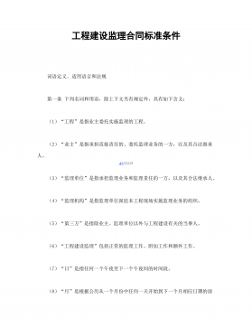
Figure 1: Sketch of the gradient estimation for VQA opti-

mization routines as shown in algorithm 1.

useful quantum advantages is given by variational

quantum algorithms (VQAs). They address the prob-

lem of estimating the ground state energy of a quan-

tum many-body Hamiltonian via a variational opti-

mization, as follows. The quantum part of VQAs

is implemented using parametrized quantum circuits

(PQCs), which are used to prepare the variational

quantum states. In order to interface it with a clas-

sical computer, the energy and the energy gradient

w.r.t. the variational parameters are typically esti-

mated. Then a classical computer, which typically

runs some gradient descent-based algorithm, is used

to minimize the energy via repeated parameter up-

dates and estimations of the energy functional.

Several challenges occur in this approach. First, on

the classical computation side, the optimization might

reach a barren plateau for the objective function [4]

or get stuck in local minima [5]. Barren plateaus

can sometimes be avoided by using smart initializa-

tions for the parameters [6]. Moreover, sophisticated

constructions of the quantum circuit family can help

to bypass such problematic regions in the parameter

space [7,8]. Local minima can at least partially be

avoided using natural gradients [9]. Second, the mea-

surement eﬀort of the quantum computer can pose a

critical bottleneck for VQAs. The reason is that

(i) many iterations steps are done in the classical

optimization,

(ii) several partial derivatives are needed for each

gradient update step,

(iii) multiple measurement settings might be needed

for the estimation of observables such as local

Hamiltonians,

(iv) quantum measurements are probabilistic, re-

arXiv:2210.06484v1 [quant-ph] 12 Oct 2022

quiring O(1/2)measurement rounds for ac-

curacy

and this can add up to a large number of total num-

ber of measurements rounds. Since quantum mea-

surements are destructive, one also needs to prepare

the entire variational state from scratch for each mea-

surement round.

In this work, we develop a new gradient estima-

tion algorithm that balances statistical and system-

atic errors which achieve a better gradient estimate

with fewer measurement rounds than conventional es-

timators. Speciﬁcally, we ﬁrst characterize both the

statistical and systematic error that arise in the esti-

mation procedure, where for the systematic error, we

introduce a Bayesian framework using prior informa-

tion and assumptions about the system to estimate it.

Then, we develop allocator methods, which for a given

measurement budget determine an optimal strategy,

namely what and how often we want to measure each

circuit conﬁguration, in order to minimize the total

error. Finally the estimator returns a gradient esti-

mate based on the measurement outcomes. A sketch

of the procedure is shown in ﬁgure 1.

The Bayesian approach takes advantage, but also

requires prior knowledge about the system. We de-

velop strategies to obtain this prior information de-

pending on the circuit depth:

(i) For short circuit, we use experimental or numer-

ical/analytical observations.

(ii) For higher depths, we use unitary 2-design prop-

erties of random circuits.

(iii) In the intermediate regime, we use an interpola-

tion of the two.

For the analysis in this paper we neglect all error

sources arising from imperfect quantum hardware and

only focus on noise due to ﬁnite measurements (i.e.

shot noise). Additionally, we assume time periodic

unitaries, meaning that, without loss of generality, the

eigenenergies of the generators can be assumed to be

integers.

Finally, we demonstrate numerically, that the

Bayesian approach outperforms previous parameter

shift rule (PSR) approaches in terms of gradient esti-

mation and VQA optimization accuracy.

1.1 Related work

There are several approaches to estimate gradients

in VQAs, notably the PSR [10,11] is able to ob-

tain unbiased gradient estimates for generators with

only two distinct eingenvalues. Further generaliza-

tions were made in Ref. [12] for a wider class of

Hamiltonians. This approach often requires ancillary

qubits or unitaries generated by commuting genera-

tors with two eigenvalues. There are also general-

izations proposed for non-commuting generators [13]

in a stochastic framework. These approaches gener-

ally require measurement settings not contained in the

VQA-ansatz, but which can be assumed to be feasible

for real hardware. There also exists unbiased estima-

tors for arbitrary periodic unitaries [14,15], where all

measurements are contained in the ansatz class.

There are also strategies [16–18] that replace the

actual observable underlying the gradient estimation

with some surrogate observables. Another research

direction has been to ﬁnd eﬃcient estimation schemes

for the whole gradient [19,20] instead of its individ-

ual partial derivatives and thus reducing the required

measurement resources.

We approach the gradient estimation diﬀerently.

Namely, we use that VQAs due to their setup expe-

rience some typical behavior, which can be analyzed

in advance and during the VQA optimization. This

allows us to also evaluate the performance of biased

estimation strategies, which under very reasonable as-

sumptions on measurement budget, can signiﬁcantly

outperform their unbiased counterparts. We use the

general framework of periodic parametrized quantum

gates [14] but believe that a similar Bayesian reason-

ing can also beneﬁt other VQA ansatz classes and gra-

dient strategies. It should therefore not be regarded

as a competitor to existing methods, but as a comple-

mentary strategy to further reduce the measurement

eﬀort of gradient estimation strategies.

1.2 Notation

We use the notation [n]:={1, . . . , n}. The Pauli ma-

trices are denoted by X,Yand Z. An operator O

acting on subsystem jof a larger quantum system is

denoted by Oj, e.g. X1is the Pauli-X-matrix acting

on subsystem 1.`p-norms including p= 0 are denoted

by k · kp. We use several symbols that are summarized

in section 8.

2 Variational quantum algorithms

In a VQA the goal is to ﬁnd parameters θsuch that

a cost function is minimized. In general, this cost

function is given by

G(θ):=hΨ0|"L

α=1

Uα(θα)#†

O"L

α=1

Uα(θα)#|Ψ0i(1)

where |Ψ0iis the initial state, Uα(θα) = e−iθαHαare

the unitary gates generated by Hαand Ois the ob-

servable encoding the optimization problem. In this

work, we are considering unitaries that are T-periodic

in θl(w.l.o.g. T= 2π), which implies that all eigen-

values of Hlare integers.

Estimating the gradient of G(θ)w.r.t. θis an im-

portant task, as most optimization algorithms are gra-

dient descent based and thus require an eﬃcient ap-

proximation of the gradient. Our strategy estimates

the gradient by the functions partial derivatives. For

this it is convenient to deﬁne the cost function at a

point shifted by a value of xin the parameter θl

Fl(x):=G(θ+xel)

=hΨ0|U†

l(x)O0Ul(x)|Ψ0i,(2)

where elis the l-th canonical basis vector and the

other layers are absorbed into the observable as O0

and the initial state as |Ψ0i. Furthermore, we used

that Ul(θl+x) = Ul(θl)Ul(x). For later reference, the

modiﬁed state and observable are

|Ψ0i="l−1

α=1

Uα(θα)#|Ψ0i, and

O0="L

α=l

Uα(θα)#†

O"L

α=l

Uα(θα)#.

(3)

The evaluation at point θ, is therefore just G(θ) =

Fl(0) and dG(θ)

dθl=F0

l(0). We will henceforth focus

only on the estimation of a single partial derivative

w.r.t. a parameter θl. In the interest of readability we

write U, and Finstead of Ul, and Fl, as well as |Ψi

and Oinstead of |Ψ0iand O0.

In this restricted view, we are now going to examine

the structure of the function F(x)more closely. The

parametrized unitary that deﬁnes this function has

the form

U(θ)=e−iθH =

nλ

i=1

Pie−iλiθ,(4)

where His a Hermitian generator and the Piare the

projectors onto the eigenspaces corresponding to the

eigenvalues {λ1, . . . , λnλ}of Hin ascending order.

Using this notation, we obtain

F(x) = hΨ|U†(x)OU(x)|Ψi

nλ

i,j=1

ei(λi−λj)xhΨ|PiOPj|Ψi,(5)

where each cij :=hΨ|PiOPj|Ψiis just a scalar. This

lets us rewrite the function as

F(x) =

nλ

i,j=1

ei(λi−λj)xcij =

nµ

k=1

ckeiµkx+c∗

ke−iµkx

nµ

k=1aksin(µkx) + bkcos(µkx),(6)

where µk∈ {|λi−λj|} are all possible eigenvalue dif-

ferences of the generator H,

ck=X

i,j:λi−λj=µk

cij (7)

and c=b+ia

2with a,b∈Rnµare Fourier coeﬃcients.

For the total number of frequencies, it follows nµ=

|{µk}| ≤ nλ

2. The derivative at x= 0 is

δ:=F0(0) =

nµ

k=1

µkak.(8)

For generators with two eigenvalues, where we can

set w.l.o.g. µk∈ {0, ν}, it has been shown that an

unbiased estimate for the partial derivative can be

obtained via

δ=νF(π

2ν)−F(−π

2ν)

2,(9)

which is known as the PSR [12].

In essence, we are going to generalize this method.

A helpful tool for this task is the antisymmetric pro-

jection

f(x) = F(x)−F(−x)

nµ

k=1

aksin(µkx).(10)

We are only considering symmetric measurement

schemes as symmetrizing an estimation method will

not make the prediction worse [14]. As such, we refer

only to the positive measurement positions xof f(x),

knowing that estimates of F(+x)and F(−x)are re-

quired to determine it. We will also omit the µ= 0

frequency, since it does not aﬀect the derivative. Ad-

ditionally, ν:=kµk∞refers to the spectral width of

the generator, meaning µ⊂[ν], since the periodic-

ity of U(x)implies that the entries of µare positive

integers.

3 Gradient estimation approach

The allocator decides the measurement resource al-

location and how to generate the estimate. In par-

ticular, we use a symmetric linear estimator of the

derivative which for a set of measurement positions

x∈[0, π)nxand number of measurements for each

position m∈Nnxreturns a gradient estimate

δ=

i=1

wiyi,(11)

where yiare the empirical estimates of f(xi)using mi

measurement rounds. Since each xirequires 2mea-

surement settings, the total number of settings is 2nx.

In the following we develop strategies to ﬁnd optimal

x,mand w.

The error

tot :=ˆ

δ−δ(12)

between our estimator guess ˆ

δand the true derivative

δis an important metric that we are going to use as

a ﬁgure of merit for choosing our estimation param-

eters. In practice, imperfections of current quantum

hardware and the lack of quantum error correction

will cause a signiﬁcant noise level when evaluating the

cost function on the quantum device. However, even

on a perfect device, the measurement process intro-

duces a shot noise error as the estimates are deter-

mined by sampling from the underlying multinomial

distribution. We denote the expectation value over

the shot noise by h · is.

The expected error under shot noise can then be

written as

htotis=

i=1

wihyiis−δ(13)

i=1

wi nµ

k=1

aksin(µkxi)!−

nµ

k=1

µkak(14)

=:(Sxw−µ)Ta,(15)

where we have used the deﬁnition (Eq. (8)) of δ, the

unbiased nature of the estimate hyiis=f(xi)and

Eq. (10) for f. We also deﬁned the matrix Sxwith

entries Sx

ki := sin(µkxi).

For the mean squared error this means

h2

totis=*nx

i=1

wiyi−δ2+s

=(Sxw−µ)Ta2+X

ihy2

iis− hyii2

s

=:2

sys +h2

statis,(16)

where the ﬁrst term describes the systematic error

resulting from the method not accurately determining

the derivative even for exact measurements and the

second term describes the statistical error arising from

measurement shot noise.

3.1 Estimating the statistical error

For the statistical error, each term hy2

iis− hyii2

sis

the variance for the measurement position xiresulting

from shot-noise errors. If the single shot variance at

position xiis σ2

i, we ﬁnd the expression

hy2

iis− hyii2

s=σ2

(17)

where miis the number of measurement rounds per-

formed for xi. For a ﬁxed measurement budget

m=Pnx

i=1 mi, the optimal measurement allocation

is given by

h2

statis= min

m:kmk1=m

i=1

σ2

=(Pnx

i=1 |wi|σi)2

with mi=m|wi|σi

Pnx

j=1 |wj|σj. If one assumes constant

shot noise σi≡σregardless of the measurement po-

sition which we will hence force do, this simpliﬁes to

h2

statis=σ2

mkwk2

1with mi=|wi|

kwk1

m . (18)

While σior σare a priori unknown, it is generally

possible to give a rough estimate of σbeforehand and

to determine an estimate of σiafter only a few mea-

surement rounds are performed. For this reason we

assume that σis a known quantity in the following

sections.

3.2 Estimating the systematic error through a

Bayesian approach

Determining the systematic error is more challenging

because it depends explicitly on the Fourier coeﬃ-

cients awhich are not known. For our analysis we

assume that the estimator will be used for an ensem-

ble of multiple diﬀerent positions θ, as one expects

to occur during a full gradient descent optimization

routine. So instead of a particular instance we want

to ﬁnd a strategy where the average total error over

the entire ensemble is minimized. The beneﬁt of this

approach is that the average only requires knowledge

of the general behavior of the Fourier coeﬃcients, not

speciﬁc values of the particular realization.

Formally, we assume that a distribution Dθover

the relevant positions θinduces a distribution of the

Fourier coeﬃcients a. One natural distribution Dθis

the uniform distribution over all parameter points θ∈

[−π, π)L, which can be motivated as a model for the

case of random initialization θ0. For an expectation

value over the distribution Dθ, we write h · iθ. In this

framework, taking the expectation value for Dθyields

h2

sysiθ=D(Sxw−µ)Ta2Eθ

= (Sxw−µ)ThaaTiθ(Sxw−µ)

=:(Sxw−µ)TCa(Sxw−µ),

(19)

meaning that the estimation of the expected squared

systematic error requires knowledge of the second mo-

ment matrix

Ca:=haaTiθ∈Rnµ×nµ.(20)

In the following, we derive properties of the of Ca

assuming the uniform distribution over θ.

First, we note that for a shift θ→θ+elzin the

layer l, the complex Fourier coeﬃcients transform as

ck→ckeiµkz, see Eq. (6). As Dθis invariant under

such a shift, we have

hckiθ=1

2πZπ

−π

hckiθdz=1

2πZπ

−π

hckeiµkziθdz= 0

implying that ckis centered around ck= 0 in expec-

tation over θ. Similarly for the second moment, we

compute

hckcpiθ=1

2πZπ

−π

hckcpiθei(µk+µp)zdz= 0 ,

hc∗

kcpiθ=1

2πZπ

−π

hc∗

kcpiθei(µk−µp)zdz=h|ck|2iθδkp ,

where δkp is the Kronecker delta. From the Fourier

expansion Eq. (6) and ak= 2 Im(ck), it follows that

hakiθ= 0

hakapiθ= 2 δkph|ck|2iθ,(21)

meaning that Cais a diagonal matrix with entries

ha2

kiθ= 2h|ck|2iθgiven by the expected squares of

the Fourier coeﬃcients.

What remains is determining ha2

kiθ. It is worth

pointing out that while underestimating ha2

kiθcan

lead to suboptimal results, even signiﬁcantly overesti-

mating the amplitudes will still outperform methods,

where no prior assumptions are made, meaning rough

estimates of ha2

kiθare already suﬃcient for good per-

formance. One way of estimating them is to use al-

ready existing empirical measurement data from pre-

vious optimization rounds or initial calibration. The

coeﬃcients can be estimated using a Fourier ﬁt. An-

other strategy involves numerically simulating smaller

system sizes and extrapolating to the actual size used

in the VQA.

If the applied unitaries in the VQA are known,

ha2

kiθcan sometimes be derived theoretically. For in-

stance in appendix D.2, we derive analytically exact

results for a VQA with a single layer (L= 1). For a

small constant circuit depth, ha2

kiθcan be computed

eﬃciently, using Monte-Carlo sampling algorithms,

even for large system sizes. This is convenient, as

the case for deep circuits, under certain assumptions,

ha2

kiθcan be approximated again using only the spec-

tral composition of the generator. This is shown in

the following.

Ergodic limit – barren plateaus

VQA optimization routines have to overcome a gen-

eral phenomenon known as barren plateaus. This term

describes the tendency of a gradient in VQAs to be

exponentially suppressed in the system size with in-

creasing circuit depth and for almost all parameters

θ. This phenomenon has been extensively studied

and while mitigation techniques are proposed [6–8],

it appears to be unavoidable, at least in the general

setup.

For the rigorous analysis of barren plateaus, it is

beneﬁcial to use the language of unitary t-designs.

Eﬀectively, with increasing circuit depth, the overall

applied gate will appear more and more like a Haar-

random unitary, with respect to which the derivative

is suppressed by the Hilbert space dimension. This

assumes that the underlying generators describe a

universal gate set. For this eﬀect to occur, we do

not need convergence to the Haar measure but con-

vergence to a unitary 2-design, which is signiﬁcantly

quicker [21,22]. For our purposes, such approximate

unitary 2-designs are suﬃcient since ha2

kiθcan be ex-

pressed as a polynomial in U, U†of degree (2,2). If

this condition is met, we can replace the expectation

value over all angles by the expectation value over all

unitaries. Hence, this condition can be summarized

by the ergodic assumption

hΓ(U(θ))iθ=ZΓ(U)dU , (22)

which holds for any polynomial Γ(U)of degree at most

(2,2) and where the integral is taken w.r.t. the Haar

probability measure on the unitary group.

Under this assumption we derive in appendix Cthat

ha2

kiθ=ξd

σ2

i≥j:µk=λi−λj

Tr[Pi/d] Tr[Pj/d](23)

with σ2

O:= Tr[O2/d]−Tr[O/d]2, where dis the Hilbert

space dimension and ξdis a constant close to 1that

depends only on d.Tr[Pi/d]is the relative multi-

plicity of the eigenvalue λi. Notably, the factor of 1

shows the exponential suppression of the derivative in

the system size, meaning that gate sets drawn from

a 2-design experience barren plateaus. For L→ ∞

this result conﬁrms the assumption that the relative

frequency of an eigenvalue diﬀerence µkin the spec-

trum of the generator determines the expected size

of its respective Fourier coeﬃcient. We will analyze

the strengths and limitations of this approach with an

example in section 5.1.

4 Allocation methods

In this section, we derive several allocation methods

for a given measurement budget. A Python imple-

mentation of these methods is available on GitHub

[23].

The estimation algorithm requires the values w,m

and x. We have already seen that making assump-

tions about the ensemble of conﬁgurations allows us

to estimate the error using the second-moment matrix

Cafrom Eq. (20) and an a priori shot noise estimate

σ2. In the following, we devise explicit measurement

procedures by making use of the knowledge of these

quantities. In section 4.1, we show that using convex

optimization procedures, one can derive an optimal

measurement strategy, which we call Bayesian linear

gradient estimator (BLGE).

In section 4.2, we then consider the case, when

the number of total measurements goes to inﬁnity.

We call this method unbiased linear gradient estima-

tor (ULGE), as it does not require access to the es-

timates of Caand σ2and yields an estimate without

systematic error. ULGE is an equivalent formulation

of a known method in literature [14]. In section 4.2.1,

we show strong similarity between ULGE and another

popular generalized PSR found in the literature [12].

Finally, in section 4.3, we restrict the number of mea-

surement positions nxto 1 and derive a strategy that

is optimal under this constraint. We call this method

single Bayesian linear gradient estimator (SLGE). We

文档加载中……请稍候！
如果长时间未打开，您也可以点击刷新试试。

下载文档到电脑，查找使用更方便

10 玖币 0人已下载

立即下载

摘要：

FastgradientestimationforvariationalquantumalgorithmsLennartBittel,JensWatty,andMartinKlieschInstituteforTheoreticalPhysics,HeinrichHeineUniversityDüsseldorf,GermanyManyoptimizationmethodsfortrainingvariationalquantumalgorithmsarebasedonestimatinggradientsofthecostfunction.Duetothestatisticalnatureo...

展开>> 收起<<

Fast gradient estimation for variational quantum algorithms.pdf

共26页,预览5页

还剩页未读，继续阅读

声明：本站为文档C2C交易模式，即用户上传的文档直接被用户下载，本站只是中间服务平台，本站所有文档下载所得的收益归上传人(含作者)所有。玖贝云文库仅提供信息存储空间，仅对用户上传内容的表现方式做保护处理，对上载内容本身不做任何修改或编辑。若文档所含内容侵犯了您的版权或隐私，请立即通知玖贝云文库，我们立即给予删除！

Fast gradient estimation for variational quantum algorithms

相关推荐

开通VIP享超值会员特权

作者详情

相关内容

热门标签

举报选择: