
Preprint PARAMETER -VARYING NEURAL ORDINARY DIFFER - ENTIAL EQUATIONS WITH PARTITION -OF-UNITY NET -
2025-05-02
0
0
1.14MB
14 页
10玖币
侵权投诉

Preprint
PARAMETER-VARYING NEURAL ORDINARY DIFFER-
ENTIAL EQUATIONS WITH PARTITION-OF-UNITY NET-
WORKS
Kookjin Lee
School of Computing and Augmented Intelligence
Arizona State University
kookjin.lee@asu.edu
Nathaniel Trask
Sandia National Laboratories
ABSTRACT
In this study, we propose parameter-varying neural ordinary differential equations
(NODEs) where the evolution of model parameters is represented by partition-
of-unity networks (POUNets), a mixture of experts architecture. The proposed
variant of NODEs, synthesized with POUNets, learn a meshfree partition of space
and represent the evolution of ODE parameters using sets of polynomials associ-
ated to each partition. We demonstrate the effectiveness of the proposed method
for three important tasks: data-driven dynamics modeling of (1) hybrid systems,
(2) switching linear dynamical systems, and (3) latent dynamics for dynamical
systems with varying external forcing.
1 INTRODUCTION
1.1 NEURAL ORDINARY DIFFERENTIAL EQUATIONS AND THEIR VARIANTS
Neural ordinary differential equations (NODEs) (Chen et al., 2018; Weinan, 2017; Haber &
Ruthotto, 2017; Lu et al., 2018) are a class of continuous-depth neural network architectures that
learn the dynamics of interest as a form of systems of ODEs:
dh(s)
ds=f(h(s); Θ),
where hdenotes a hidden state, srepresents a continuous depth, and the velocity function fis
parameterized by a feed-forward neural network with learnable model parameters Θ.
As pointed out in (Massaroli et al., 2020), the original NODE formulation (Chen et al., 2018), is
limited to incorporate the depth variable sinto dynamics as it is, e.g., by concatenating sand h,
which are then fed to f(h, s; Θ), rather than constructing the map s7→ Θ(s). Recent studies inves-
tigate strategies to extend NODEs to be depth-variant. ANODEV2 (Zhang et al., 2019) proposes a
hypernetwork-type approach which builds a coupled system of NODEs, where one NODE defines
an evolution of state variables, while another NODE defines an evolution of model parameters. In
(Massaroli et al., 2020), stacked NODEs and Galerkin NODEs (GalNODEs) have been proposed
where the evolution of model parameters are modeled as piecewise constants and a set of orthogonal
basis, respectively. The idea of spectrally modeling model parameters has been further extended to
enable basis transformation leading to stateful layers and compressible model parameters (Queiruga
et al., 2021).
In this work, following the work by (Massaroli et al., 2020) which has proposed two depth-variant
NODEs: stacked NODEs (i.e., a piecewise constant representation of model parameters, e.g., Fig-
ure 1a) and Galerkin NODEs (i.e., spectral representation of model parameters, e.g., Figure 1b).
Inspired by these two variants, we propose an a combination of stacked and Galerkin NODEs lead-
ing to spectral-element-like (Patera, 1984) or hp-finite-element-like (Solin et al., 2003) methods,
which we denote by Partition-of-Unity NODEs (POUNODEs, e.g., Figure 1c). We decompose the
domain of model parameters (e.g., depth) into disjoint learnable partitions, with model parameters
approximated on each as polynomials.
1
arXiv:2210.00368v1 [cs.LG] 1 Oct 2022

Preprint
(a) Stacked NODE (b) Galerkin NODE (c) POUNODE
Figure 1: An illustrative example depicting evolution of model parameters for Stacked NODE,
Galerkin NODE, and the proposed POUNODE. Models are trained to perform the binary classifica-
tion task of two concentric circles.
Our main contributions include 1) development of an hp-element-like method for representing the
evolution of model parameters of NODEs and 2) to showcase the effectiveness of POUNODEs
with three different important applications: learning hybrid systems, switching linear dynamics, and
latent-dynamics modeling with varying external factor.
2 POUNETS INTO NODES
We begin by introducing partition-of-unity networks (POUNets) (Lee et al., 2021b), which a partic-
ular type of deep neural network developed for approximating functions with exponential conver-
gence. POUNets automatically learn partitions of the domain and simultaneously compute the co-
efficients of polynomials associated in each partition. Then we introduce a method to use POUNets
for representing the evolution of model parameters for NODEs.
2.1 PARTITION-OF-UNITY NETWORKS
Several recent works (He et al., 2018; Yarotsky, 2017; 2018; Opschoor et al., 2019; Daubechies
et al., 2019) on approximation theory of deep neural networks (DNNs) investigate the role of width
and depth to the performance of DNNs and have theoretically proved the existence of model pa-
rameters of DNNs that emulate algebraic operations, a partition of unity (POU), and polynomials
to exponential accuracy in the depth of the network. That is, in theory, with a sufficiently deep
architecture, DNNs should be able to learn a spectrally convergent hp-element space by construct-
ing a POU to localize polynomial approximation without a hand-tailored mesh. As has seen in
(Fokina & Oseledets, 2019; Adcock & Dexter, 2020; Lee et al., 2021b), however, such convergent
behaviours in practice are not realized due to many reasons (e.g., gradient-descent-based training).
In (Lee et al., 2021b), a novel neural network architecture, POUNets, has been proposed, which
explicitly incorporates a POU and polynomial elements into a neural network architecture, leading
to exponentially-convergent DNNs.
(a) Partitions (b) Quadratic wave
Figure 2: Learned partitions (left) and
predictions (cian dashed) depicted with
the ground truth target function (black
solid).
Mathematically, a POU can be defined as Φ(x) =
{φi(x)}npart
i=1 satisfying Piφi(x) = 1 and φi≤0for all
x. Then POUNets can be represented as
yPOU(x) =
npart
X
i=1
φi(x;π)
dim(V)
X
j=1
αi,j φj(x),
where V=span({ψj}), typically taken as the
space of polynomials of order m, and Φ(x;π) =
[φ1(x;π), . . . , φnpart (x;π)] is parameterized by a neural
network with the model parameters π. To ensure the prop-
erties of the partition-of-unity, the output layer of the neu-
ral network Φis designed to produce positive and normal-
ized output (i.e., φi(x;π)≥0and Piφi(x;π) = 1).
Figure 2 depicts an example of regressing a quadratic
wave with a POUNet, where standard MLPs exhibit poor
2

Preprint
performance: the left panel shows the learned partitions and the right panel shows the ground truth
target function (solid black) and the prediction (dashed cian). In each partition, a set of monomials
with the maximal degree 2 is fitted optimally by solving local linear least-squares problems.
2.2 PARTITION-OF-UNITY-BASED NEURAL ORDINARY DIFFERENTIAL EQUATIONS
Now, we introduce the proposed partition-of-unity-based neural ordinary differential equations,
where the model parameters are represented as a POUNet: Θ(s)∈RnΘ:
Θ(s;α, π) =
npart
X
i=1
φi(s;π)pi(s) =
npart
X
i=1
φi(s;π)
npoly
X
j=1
αi,j ψj(s),(1)
where sdenotes a set of variables whose domains are expected to have a set of partitions (e.g.,
scan be a depth variable in depth-continuous neural network architectures), φi(s;π)∈Rde-
notes a partition of unity network, parameterized by π,ψj(s)∈Rdenotes a polynomial basis,
and α·,j ∈RnΘdenote the polynomial coefficients. Thus, collectively, there is a set of parameters
α= (α1, . . . , αnpart )with αi= [αi,1· · · , αi,npoly ]∈Rnθ×npoly . In the following, we present a couple
example cases of the types of the variables s.
Temporally varying dynamics / depth variance As in the typical settings of NODEs, when an
MLP is considered to parameterize the velocity function, f(·; Θ), the model parameters can be rep-
resented as a set of constant-valued variables, Θ = {(W`,b`)}L
`=1, where W`and b`denote weights
and biases of the `-th layer. As opposed to the depth-invariant NODE parameters Θ, POUNODEs
represent depth-variant NODEs (or non-autonomous dynamical systems) by setting the model pa-
rameters as
Θ(t) = {(W`(t),b`(t))}L
`=1,
where tdenotes the time variable or the depth of the neural network and represent, and by represent-
ing Θ(t)as a POUNet as in Eq. (1) with s=t.
Spatially varying dynamics Another example dynamical systems that can be represented by
POUNODEs is a class of dynamical systems whose dynamics modes are defined differently on
different spatial regions. In this case, the model parameters can be set as spatially-varying ones:
Θ(x) = {(W`(x),b`(x))}L
`=1.
and can be represented as a POUNet as in Eq. (1) with s=x.
Remark 2.1. Although not numerically tested in this study, the idea of representing the evolution
of model parameters via POUNets can be applied to different neural network architectures, e.g.,
POU-Recurrent Neural Networks (POU-RNNs).
3 USE CASES
This section exhibits example use cases where the benefits of using POUNODE can be pronounced.
All implementations are based on PYTORCH (Paszke et al., 2019) and the TORCHDIFFEQ library
(Chen et al., 2018) for the NODEs capability.
For all following experiments, we consider a POUNet, Φ = {φi}npart
i=1, based on a radial basis function
(RBF) network (Broomhead & Lowe, 1988; Billings & Zheng, 1995); for each partition, there is an
associated RBF layer, defined by its center and shape parameter, and then the output of the RBF
layers is normalized to satisfy the partition-of-unity property (refer to Appendix for more details).
3.1 SYSTEM IDENTIFICATION OF A HYBRID SYSTEM
As a first set of use cases, we apply POUNODEs for data-driven dynamics modeling. In particular,
we aim to learn a dynamics model for a hybrid system, where the different dynamics models are
mixed in a single system: a system consisting of multiple smooth dynamical flows (SDFs), each
of which is interrupted by sudden changes (e.g., jump discontinuities or distributional shifts) (Van
Der Schaft & Schumacher, 2000).
3

摘要:
展开>>
收起<<
PreprintPARAMETER-VARYINGNEURALORDINARYDIFFER-ENTIALEQUATIONSWITHPARTITION-OF-UNITYNET-WORKSKookjinLeeSchoolofComputingandAugmentedIntelligenceArizonaStateUniversitykookjin.lee@asu.eduNathanielTraskSandiaNationalLaboratoriesABSTRACTInthisstudy,weproposeparameter-varyingneuralordinarydifferentialequa...
声明:本站为文档C2C交易模式,即用户上传的文档直接被用户下载,本站只是中间服务平台,本站所有文档下载所得的收益归上传人(含作者)所有。玖贝云文库仅提供信息存储空间,仅对用户上传内容的表现方式做保护处理,对上载内容本身不做任何修改或编辑。若文档所含内容侵犯了您的版权或隐私,请立即通知玖贝云文库,我们立即给予删除!
相关推荐
-
政治理论应知应会 100 题VIP免费
 2024-12-12 394
 -
2025年中央机关及其直属机构录用公务员考试 行政职业能力测验(地市级)(经典模考卷三)解析VIP免费
 2024-12-12 49
 -
021水平面内的圆周运动(圆锥摆模型)及其临界问题 精讲精练-2022届高三物理一轮复习疑难突破微专题VIP免费
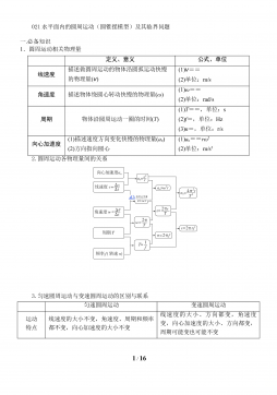
 2025-01-04 48
 -
21学位英语:从句考点真题VIP免费
 2025-04-08 7
 -
19学位英语:2010年阅读理解分析VIP免费
 2025-04-08 4
 -
[16] 学位英语:2007年阅读理解分析VIP免费
 2025-04-08 5
 -
[15] 学位英语:2006年阅读理解分析VIP免费
 2025-04-08 11
 -
[14] 学位英语:2005年阅读理解分析VIP免费
 2025-04-08 13
 -
[13] 学位英语:2004年阅读理解分析VIP免费
 2025-04-08 10
 -
[10] 学位英语:长难句拆分(二)VIP免费
 2025-04-08 11
分类:图书资源
价格:10玖币
属性:14 页
大小:1.14MB
格式:PDF
时间:2025-05-02
作者详情
相关内容
-
[16] 学位英语:2007年阅读理解分析
分类:高等教育
时间:2025-04-08
标签:无
格式:DOC
价格:5.9 玖币
-
[15] 学位英语:2006年阅读理解分析
分类:高等教育
时间:2025-04-08
标签:无
格式:DOC
价格:5.9 玖币
-
[14] 学位英语:2005年阅读理解分析
分类:高等教育
时间:2025-04-08
标签:无
格式:DOC
价格:5.9 玖币
-
[13] 学位英语:2004年阅读理解分析
分类:高等教育
时间:2025-04-08
标签:无
格式:DOC
价格:5.9 玖币
-
[10] 学位英语:长难句拆分(二)
分类:高等教育
时间:2025-04-08
标签:无
格式:DOC
价格:5.9 玖币

