Policy-Guided Lazy Search with Feedback for Task and Motion Planning Mohamed Khodeir1Atharv Sonwane2Ruthrash Hari3Florian Shkurti1 Abstract PDDLStream solvers have recently emerged as

2025-05-02 0 0 4.25MB 8 页 10玖币

侵权投诉

Policy-Guided Lazy Search with Feedback for Task and Motion Planning

Mohamed Khodeir1Atharv Sonwane2Ruthrash Hari3Florian Shkurti1

Abstract— PDDLStream solvers have recently emerged as

viable solutions for Task and Motion Planning (TAMP) problems,

extending PDDL to problems with continuous action spaces.

Prior work has shown how PDDLStream problems can be

reduced to a sequence of PDDL planning problems, which

can then be solved using off-the-shelf planners. However,

this approach can suffer from long runtimes. In this paper

we propose

LAZY

, a solver for PDDLStream problems that

maintains a single integrated search over action skeletons, which

gets progressively more geometrically informed, as samples of

possible motions are lazily drawn during motion planning. We

explore how learned models of goal-directed policies and current

motion sampling data can be incorporated in

LAZY

to adaptively

guide the task planner. We show that this leads to signiﬁcant

speed-ups in the search for a feasible solution evaluated over

unseen test environments of varying numbers of objects, goals,

and initial conditions. We evaluate our TAMP approach by

comparing to existing solvers for PDDLStream problems on a

range of simulated 7DoF rearrangement/manipulation problems.

Code can be found at

https://rvl.cs.toronto.edu/

learning-based-tamp.

I. INTRODUCTION

Task and motion planning (TAMP) problems are challeng-

ing because they require reasoning about both discrete and

continuous decisions that are interdependent. TAMP solvers

typically decompose the problem by using a symbolic task

planner that searches over discrete abstract actions, such as

which object to interact with or what operations are applicable,

and a motion planner which attempts to ﬁnd the continuous

parameters that ground those abstract actions, for instance

grasp poses and robot conﬁgurations. The motion planner

informs the task planner when backtracking is necessary.

Thus, the interplay between abstract task planning and low-

level motion planning has a signiﬁcant effect on both runtime

and percentage of problems solved.

In this work, we provide a signiﬁcantly improved PDDL-

Stream [

] solver (

LAZY

) for task and motion planning

problems, which learns to plan from experience and adapts

based on current execution data. The motion planner of

our solver provides feasibility updates to a priority/guidance

function that is used to inform action selection by the symbolic

task planner.

LAZY

plans optimistically and lazily (deferring

motion sampling until an action skeleton is found), and

maintains a single uniﬁed search tree, as opposed to solving

a sequence of PDDL problems over a growing set of facts,

as was done in [1] and its current variants.

Robot Vision and Learning Lab, University of Toronto Robotics Institute.

2Dept. of Computer Science, University of BITS Pilani

Dept. of Mathematical and Computational Sciences, University of Toronto

{m.khodeir, ruthrath.hari}@mail.utoronto.ca,

atharvs.twm@gmail.com, florian@cs.toronto.edu

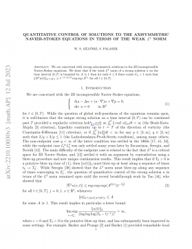
Fig. 1: Top Left: Simulated evaluation tasks in Clutter environment. Top Right:

Real-world manipulation problems using two 7DoF robot arms. Bottom: A

ﬂowchart illustrating the high level components of our approach.

A core component of our method is a goal-conditioned

policy over high-level actions, which we learn using behaviour

cloning on past planning demonstrations. This policy is treated

as a priority function, which guides the action skeleton

search performed by the task planner towards promising

abstract action sequences. While this can often eliminate the

need for backtracking altogether, the policy may still predict

geometrically infeasible actions in more challenging TAMP

problems. We therefore show how the predictions of this

priority function can be updated online in response to failed

samples in motion planning, allowing successive iterations of

the task planner to focus the search on more feasible action

sequences. The result is a policy-guided bi-level search for

TAMP problems, which improves online from experience and

past data, and demonstrates impressive planning performance

on unseen environments from a test distribution, while being

trained with only a few hundred demonstrations.

Our main contributions are: (1) A lazy search framework for

PDDLStream problems, which maintains a single search tree

over symbolic plan skeletons. (2) A method for incorporating

a learned policy over symbolic actions into sampling-based bi-

level search, and efﬁciently updating it online using feedback

from motion planning. (3) A concrete parametrization of

this goal conditioned policy as a Graph Attention Network

(GAT) which incorporates both high-level and low-level state.

We empirically evaluate our proposed method compared to

existing approaches for sampling-based TAMP, such as [

]

and show signiﬁcant (37%) improvement in the number of

unseen problems solved within the allotted planning time.

II. BACKGROUND: PDDL AND PDDLSTREAM

We adopt PDDLStream [

] as the formalism for expressing

TAMP problems. A PDDLStream domain

(P,A,Ψ)

deﬁned by predicates P, actions A, and streams Ψ.

arXiv:2210.14055v4 [cs.RO] 23 Aug 2023

At a high level, predicates are boolean valued n-ary

functions which indicate the presence of particular relations

among their variables. For instance, the predicate

isOn

may

indicate that the object in its ﬁrst argument is on top of the

object in its second. When a predicate is applied to speciﬁc

objects (e.g. isOn(A, B)), we refer to it as a “fact”.

Actions deﬁne the legal state transitions in the planning

problem. They are deﬁned by a set of parameters, a set of

preconditions which deﬁne facts on those parameters which

must hold in order for the action to be applicable, and effects

that determine which facts about the parameters are added

or removed following the application of the action.

The set of streams,

, distinguishes a PDDLStream

domain from traditional PDDL. Streams are conditional

generators which yield objects that satisfy speciﬁc constraints

conditioned on their inputs. Formally, a stream,

, is deﬁned

by input and output parameters

¯x

¯o

, a set of facts

domain(s)

and a set of facts

certified(s)

domain(s)

is the set of facts

that must evaluate to true for an input tuple

¯x

to be valid.

This ensures the correct types of objects (e.g., conﬁgurations,

poses etc.) are provided to the generators.

certified(s)

are

facts about

¯x

and

¯o

that will be true of any outputs

¯o

that the

stream generators produce. Streams can be applied recursively

to generate a potentially inﬁnite set of objects and their

associated facts, starting from those in

. They can also be

thought of as declaratively specifying constraints between

their inputs and outputs. Finally, each stream comes with a

black-box procedure which, given input values

¯x

, produces

samples

¯o

which satisfy those constraints. We use the term

stream evaluation to refer to the act of querying this sampler.

The PDDLStream domain

(P,A,Ψ)

deﬁnes a language in

which to pose speciﬁc problems. An instance of a planning

problem in this domain is deﬁned by specifying the initial

state

which is simply a set of facts using predicates

that

describe the initial scene, and the goal

and

implicitly

deﬁne a set of initial objects over which facts in those sets

are stated. A solution to a problem instance consists of a

sequence of action instances which result in a state in which

is satisﬁed. Note that many of the parameters in a solution

may need to be produced using the streams and initial objects.

Predicates in classical PDDL problems can be classiﬁed as

either “static” or “ﬂuent” depending on whether they appear

in the effects of any action. Static predicates are used to deﬁne

types (e.g.

isTable(x)

) or immutable relations between

objects (e.g.

isSmaller(x, y)

). Fluent predicates, on the

other hand, are those which can be changed by actions (e.g.

isOn(x, y)

). By deﬁnition, streams are only allowed to

certify “static” predicates (e.g.

isGraspPose(x)

). There-

fore, in PDDLStream problems, we can further categorize

static predicates based on whether they are produced by

streams or are simply given in the initial conditions

. We

call the former stream-certiﬁed preconditions.

We use the notation

⃗a

to refer to an “action skeleton”,

which is a sequence of discrete, high-level action instances

with continuous parameters left as variables (for instance,

grasp poses and placement poses). See Fig. 3 for an example

of a two-step action skeleton. We denote a speciﬁc assign-

ment/grounding of continuous parameters as

⃗

, and refer to

the grounded plan as

⃗a(⃗

θ)

. Similarly, we use

and

a(θ)

to refer to individual actions and their grounding.

III. OUR APPROACH

A. Lazy Bi-Level Search

Our overall framework is a bi-level search, similar to prior

work on task and motion planning ([

], [

]). In every iteration,

we search for an action skeleton

⃗a

. This outer search for an

action skeleton is guided by a priority function

, which

assigns a lower value to more desirable actions. We describe

possible choices for how

is deﬁned in section III-B and

elaborate on the details of skeleton search in section III-C.

Once an action skeleton is found in the outer search,

we perform the inner search for grounding its continuous

parameters

⃗

. We refer to this as skeleton reﬁnement, and

elaborate on it in section III-D. The overall procedure

terminates when reﬁnement is successful, in which case a

complete trajectory is returned. Otherwise, the result of the

previous reﬁnement is used to update the priority function

and the next iteration begins, yielding a potentially different

action skeleton. We refer to the process of incorporating the

result of reﬁnement into the priority function used by the

outer search as feedback and detail a number of possible

implementations in section III-E. The search fails to solve a

given problem if the allotted planning time runs out before a

trajectory is found. This overall framework is summarized in

Algorithm 1 and illustrated in Figure 1.

B. Skeleton Search Routines and their Priority Functions

There are many possible choices for the skeleton

routine and its associated priority function

leading to

algorithms with different characteristics. In this work, we

consider two implementations of

: the ﬁrst is a simple

best-ﬁrst search and the second is a beam search. Intuitively,

decreasing the value of the beam width parameter in beam

search allows us to create greedier search algorithms at the

cost of potentially pruning out solution branches.

We also consider two implementations of

: ﬁrst, the

familiar A* priority function (

f(n) = g(n) + h(n)

), which

we use to incorporate off-the-shelf domain-agnostic heuristics

from prior work [

]. Note that this option allows our algorithm

to work well without a learned policy, using existing domain-

agnostic search heuristics in place of

. We make use of this

for data collection, and as a baseline in evaluation.

Second, we build on ideas from Levin Tree Search

(LevinTS) [

] as a way to incorporate a policy to guide

the search while maintaining guarantees about completeness

and search effort of the symbolic planner that relate to

the quality of the policy. We assume that we are given a

policy

π(a|s, G)

which predicts a probability distribution

over applicable discrete actions (i.e. logical state transitions)

conditioned on a logical state

s∈ S

and goal

G ⊂ S

, where

Sis the set of all logical states.

We distinguish between a state in the search space and a

node in the search tree by using the symbol

to denote the

former and

to denote the latter. A node corresponds to a

文档加载中……请稍候！
如果长时间未打开，您也可以点击刷新试试。

下载文档到电脑，查找使用更方便

10 玖币 0人已下载

立即下载

摘要：

Policy-GuidedLazySearchwithFeedbackforTaskandMotionPlanningMohamedKhodeir1AtharvSonwane2RuthrashHari3FlorianShkurti1Abstract—PDDLStreamsolvershaverecentlyemergedasviablesolutionsforTaskandMotionPlanning(TAMP)problems,extendingPDDLtoproblemswithcontinuousactionspaces.PriorworkhasshownhowPDDLStreampro...

展开>> 收起<<

Policy-Guided Lazy Search with Feedback for Task and Motion Planning Mohamed Khodeir1Atharv Sonwane2Ruthrash Hari3Florian Shkurti1 Abstract PDDLStream solvers have recently emerged as.pdf

共8页,预览2页

还剩页未读，继续阅读

声明：本站为文档C2C交易模式，即用户上传的文档直接被用户下载，本站只是中间服务平台，本站所有文档下载所得的收益归上传人(含作者)所有。玖贝云文库仅提供信息存储空间，仅对用户上传内容的表现方式做保护处理，对上载内容本身不做任何修改或编辑。若文档所含内容侵犯了您的版权或隐私，请立即通知玖贝云文库，我们立即给予删除！

Policy-Guided Lazy Search with Feedback for Task and Motion Planning Mohamed Khodeir1Atharv Sonwane2Ruthrash Hari3Florian Shkurti1 Abstract PDDLStream solvers have recently emerged as

相关推荐

开通VIP享超值会员特权

作者详情

相关内容

热门标签

举报选择: