
An Order Statistics PostMortem on LIGOVirgo GWTC2 Events Analyzed with Nested Sampling_2
2025-04-27
0
0
770.96KB
8 页
10玖币
侵权投诉

RESEARCH ARTICLE
www.ann-phys.org
An Order Statistics Post-Mortem on LIGO–Virgo GWTC-2
Events Analyzed with Nested Sampling
Talya Klinger* and Michalis Agathos
The data analysis carried out by the LIGO–Virgo collaboration on
gravitational-wave events utilizes nested sampling to compute Bayesian
evidences and posterior distributions for inferring the source properties of
compact binaries. With poor sampling from the constrained prior, nested
sampling algorithms may misbehave and fail to sample the posterior
distribution faithfully. Fowlie et al. (2020) outlines a method of validating the
performance of nested sampling, or identifying pathologies such as plateaus
in the parameter space, using likelihood insertion order statistics. Here, this
method is applied to nested sampling analyses of all events in the first and
second gravitational wave transient catalogs (GWTC-1 and GWTC-2) of the
LIGO–Virgo collaboration. The insertion order statistics are tested for
uniformity across 45 events in the catalog and it is found that, with a few
exceptions that have negligible effect on the final posteriors, the data from the
analysis of events in the catalog is consistent with unbiased prior sampling.
There is, however, weak evidence against uniformity at the catalog-level
meta-test, yielding a Kolmogorov–Smirnov meta-p-value of 1.44 ×10⁻³.
1. Introduction
Since the first direct detection of gravitational waves (GWs) in
2015,[1] the LIGO–Virgo collaboration (LVC) has published the
detection of tens of GW signals emitted by coalescing black-
hole and neutron-star binaries, in the three observing runs car-
ried out so far (O1, O2, and O3).[2–4] In gravitational-wave data
analysis, parameter estimation is the process of inferring the
source properties of signals which have already been identified as
T. Klinger
Cardiff University School of Physics and Astronomy
5 The Parade, Newport Road, Cardiff CF24 3AA, UK
E-mail: talyaklinger@gmail.com
M. Agathos
DAMTP
Centre for Mathematical Sciences
University of Cambridge
Wilberforce Road, Cambridge CB3 0WA, UK
M. Agathos
Kavli Institute for Cosmology Cambridge
Madingley Road, Cambridge CB3 0HA, UK
The ORCID identification number(s) for the author(s) of this article
can be found under https://doi.org/10.1002/andp.202200271
© 2022 The Authors. Annalen der Physik published by Wiley-VCH
GmbH. This is an open access article under the terms of the Creative
Commons Attribution License, which permits use, distribution and
reproduction in any medium, provided the original work is properly cited.
DOI: 10.1002/andp.202200271
gravitational waves produced by com-
pact binaries. Bayesian inference meth-
ods are employed to fit waveform models
to data, using algorithms designed for ef-
ficiently sampling high-dimensional pa-
rameter spaces. One such algorithm is
nested sampling, a method for efficiently
computing Bayesian evidences as well as
posterior probability distributions, intro-
duced by Skilling in 2006[5] (for a review,
see ref. [6]). Here, we use a new method
of statistically verifying nested sampling
output, the insertion order cross-check
developed by Fowlie et al.,[7] to test for
biased nested sampling in the LVC’s
gravitational-wave data analysis.
The LVC uses nested sampling along-
side Markov Chain Monte Carlo (MCMC)
and occasionally RIFT[8] to obtain pos-
terior distributions in parameter esti-
mation. These algorithms serve nec-
essary and complementary purposes.
While the LVC’s implementation of MCMC converges faster
for signals with long inspiral times, and RIFT allows for di-
rect comparison to numerical relativity, they do not directly
compute evidence, delivering only the normalized posterior
and requiring further statistical calculations to estimate the ev-
idence, introducing significant statistical errors. Nested sam-
pling computes the evidence directly, allowing for greater
accuracy.
In the LSC algorithm library (LAL), nested sampling was orig-
inally implemented in the LALInference package.[9,10] During the
third observing run (O3), the LVC (now LVK) Collaboration grad-
ually shifted its main data analysis pipelines to a newer Bayesian
inference library bilby,[11] a Python-based modular code which
combines LAL’s libraries for data infrastructure and waveform
modeling with third-party nested samplers. The insertion order
cross-check defined later in this paper has already been imple-
mented in many bilby samplers, including CPNest,[12] nessai,[13]
and UltraNest.[14] However, the first two observing runs, O1 and
O2, and the first half of the third observing run, O3a, were ana-
lyzed using LALInference alone. In this work, we utilize the inser-
tion order cross-check to perform a post-mortem analysis on all
nested sampling output for GW events in O1, O2, and O3a, eval-
uating the validity of parameter estimation results for the LVC’s
event catalogs GWTC-1 and GWTC-2.[15]
This article is structured as follows. In Section 2 we briefly
describe the nested sampling algorithm and the insertion order
statistics we use to estimate the validity of the LVC analyses. We
then describe our implementation for the parameter-estimation
Ann. Phys. (Berlin)2022, 2200271 2200271 (1 of 8) © 2022 The Authors. Annalen der Physik published by Wiley-VCH GmbH

www.advancedsciencenews.com www.ann-phys.org
dataset output by LALInference in Section 4 and present the re-
sults on the GW events in Section 5. Concluding remarks are
given in Section 6.
2. Insertion Order Statistics in Nested Sampling
2.1. Nested Sampling
For a given GW event associated with the coalescence of a com-
pact binary, we can describe its source properties by a parame-
ter vector 𝜃∈Θ,whereΘdenotes the corresponding parameter
space, including the mass and spin of each component, the dis-
tance to the source, its sky-location and orientation angles, time,
and phase of coalescence, as well as any additional parameters
relating to matter properties in case of a neutron star, orbital ec-
centricity, etc. Given the observed data D, our aim is to infer the
parameters 𝜃of the source, i.e. estimate the posterior distribu-
tion P(𝜃|D, ) under the assumption that our background infor-
mation about the nature of the source, the behavior of our de-
tectors and the validity of GR as the underlying theory is correct.
In Bayesian statistics, this amounts to updating our prior ex-
pectations quantified by P(𝜃|) by making appropriate use of
Bayes’ theorem
P(D|𝜃,)×P(𝜃|)=P(D|)×P(𝜃|D, )(1)
L(𝜃)×𝜋(𝜃)d𝜃=Z×p(𝜃)d𝜃
L(𝜃)=P(D|𝜃,), known as the likelihood function, and 𝜋(𝜃)=
P(𝜃|), the prior, give the desired quantities Z=P(D|), the evi-
dence and p=P(𝜃|D, ), the posterior. Computing the likelihood
function (the probability density for observing data D, given the
model and the true values of the parameters) requires models
for both the detector signal and noise—in LIGO’s case, LALSim-
ulation can generate a waveform model for the signal, while the
noise for each detector is assumed to be Gaussian and is charac-
terized by a power spectral density (PSD) which is pre-estimated
based on a stretch of data around the time of the event.[15] Infor-
mation from all detectors in operation is combined into a coher-
ent network likelihood which is the product of individual detec-
tor likelihoods.[10] The task of efficiently sampling the parameter
space to map the likelihood function, is carried out by the nested
sampling algorithm.
The evidence Z—the probability of observing the measured
data, given the model—is defined as
Z=∫L(𝜃)𝜋(𝜃)d𝜃(2)
This is an important quantity in Bayesian data analysis, as
the evidences produced by different models can be directly com-
pared. Hence, the evidence can be used to rank competing hy-
potheses and quantify how much a given model is supported by
the data. dX=𝜋(𝜃)d𝜃is known as the element of prior mass. If
the prior mass contained by a likelihood contour
X(𝜆)=∫L(𝜃)>𝜆
𝜋(𝜃)d𝜃(3)
is known, the evidence can be written as a 1D integral,
Z=∫1
0
L(X)dX(4)
which is more computationally manageable than integrating
across a high-dimensional parameter space Θ.
Nested sampling is a method for computing evidence that
takes advantage of this formulation, relying on the statistical
properties of prior sampling to provide a fast and accurate es-
timate of the prior mass at each integration step.
2.2. Summary of the Nested Sampling Algorithm
Nested sampling relies on sampling from the constrained prior:
points from the prior with likelihood higher than some mini-
mum value. As points from the constrained prior are sampled
and discarded throughout the algorithm, the samples used at
each step are called live points.
The nested sampling algorithm proceeds as follows:
1. Choose the number of live points nlive and sample nlive ini-
tial points from the constrained prior. Also, set an evidence
threshold 𝜖.
2. Identify the live point with the lowest likelihood L∗
i. Discard
the live point and record its likelihood.
3. Sample a new live point from 𝜋(𝜃) with L>L∗
i. At this stage,
the prior volume compresses exponentially, giving prior vol-
ume Xi≈exp(−1∕nlive) on the ith step (the proof is nontrivial,
see ref. [5]).
4. Integrate the evidence Ziusing L∗
iand Xi.
5. Repeat steps (2)–(4) until a stopping condition is reached:
LmaxXi∕Zi<e𝜖,whereLmax is the highest likelihood discov-
ered so far, Xiis the prior volume inside the current iso-
likelihood contour L∗
i,andZiis the current estimate of the
evidence. For LALInference,𝜖=0.1; essentially, if all the live
points were to have the maximum discovered likelihood, the
evidence would only change by a factor of less than 0.1.[10]
Nested sampling requires faithful sampling from the con-
strained prior to produce accurate evidences and posteriors. In
practice, sampling from the entire prior and accepting only
points with high enough likelihood is impractically slow, be-
cause the volume of acceptable points decreases exponentially
in time. So, most implementations of nested sampling sample
from a restricted region of parameter space drawn around the
live points. LALInference, in particular, generates samples by an
MCMC chain from a randomly chosen previous livepoint, and
choosing the length of the MCMC chain is a tradeoff between
speed and accuracy.[10]
If the restricted region is too small or the MCMC chains too
short, the constrained prior may not fully cover the iso-likelihood
contour, violating the fundamental assumptions of nested sam-
pling. Plateaus—regions of constant L(𝜃)—also violate the as-
sumptions of nested sampling, causing live points to be nonuni-
formly distributed in X.
2.3. Insertion Order Crosscheck
The insertion index is the position where an element must be
inserted in a sorted list to preserve order. More concretely, if xis
a sorted list and there exists a sample ysuch that
xi−1<y<xi(5)
Ann. Phys. (Berlin)2022, 2200271 2200271 (2 of 8) © 2022 The Authors. Annalen der Physik published by Wiley-VCH GmbH

摘要:
展开>>
收起<<
RESEARCHARTICLEwww.ann-phys.orgAnOrderStatisticsPost-MortemonLIGO–VirgoGWTC-2EventsAnalyzedwithNestedSamplingTalyaKlinger*andMichalisAgathosThedataanalysiscarriedoutbytheLIGO–Virgocollaborationongravitational-waveeventsutilizesnestedsamplingtocomputeBayesianevidencesandposteriordistributionsforinfer...
声明:本站为文档C2C交易模式,即用户上传的文档直接被用户下载,本站只是中间服务平台,本站所有文档下载所得的收益归上传人(含作者)所有。玖贝云文库仅提供信息存储空间,仅对用户上传内容的表现方式做保护处理,对上载内容本身不做任何修改或编辑。若文档所含内容侵犯了您的版权或隐私,请立即通知玖贝云文库,我们立即给予删除!
相关推荐
-
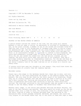
Michael Moorcock - Elric 6 - StormbringerVIP免费
 2024-12-08 19
 -
Michael Crichton - PreyVIP免费
 2024-12-08 22
 -
Mercedes Lackey - WintermoonVIP免费
 2024-12-08 19
 -
Mercedes Lackey - SE 1- Born To RunVIP免费
 2024-12-08 18
 -
Mercedes Lackey - Heralds of Valdemar 1 - Arrows Of The QueeVIP免费
 2024-12-08 24
 -
Melville, Herman - TypeeVIP免费
 2024-12-08 31
 -
MaryJanice Davidson - [Betsy 5] - Undead and Unpopular (v1.0)VIP免费
 2024-12-08 34
 -
Marion Zimmer Bradley - Darkover - The Heirs of HammerfellVIP免费
 2024-12-08 38
 -
MacDonnell, J E - 096 - Execute!VIP免费
 2024-12-08 23
 -
Lovecraft, H P - The Dream Quest Of Unknown KadadthVIP免费
 2024-12-08 41
分类:图书资源
价格:10玖币
属性:8 页
大小:770.96KB
格式:PDF
时间:2025-04-27
作者详情

相关内容
-
2015年6月英语四级真题答案及解析(卷二)
分类:外语学习
时间:2025-05-02
标签:无
格式:PDF
价格:5.8 玖币
-
2015年6月英语四级真题答案及解析(卷三)
分类:外语学习
时间:2025-05-02
标签:无
格式:PDF
价格:5.8 玖币
-

2016年12月六级(第二套)真题
分类:外语学习
时间:2025-05-02
标签:无
格式:PDF
价格:5.8 玖币
-

2016年12月六级(第三套)真题
分类:外语学习
时间:2025-05-02
标签:无
格式:PDF
价格:5.8 玖币
-

2016年12月六级(第一套)真题
分类:外语学习
时间:2025-05-02
标签:无
格式:PDF
价格:5.8 玖币

