Two-parameter sums signatures and corresponding quasisymmetric functions Joscha Diehl Leonard Schmitz

2025-05-06 0 0 1.2MB 61 页 10玖币

侵权投诉

Two-parameter sums signatures and

corresponding quasisymmetric functions

Joscha Diehl Leonard Schmitz

University of Greifswald

Quasisymmetric functions have recently been used in time series analysis

as polynomial features that are invariant under, so-called, dynamic time

warping. We extend this notion to data indexed by two parameters and

thus provide warping invariants for images. We show that two-parameter

quasisymmetric functions are complete in a certain sense, and provide a

two-parameter quasi-shuﬄe identity. A compatible coproduct is based on

diagonal concatenation of the input data, leading to a (weak) form of Chen’s

identity.

Keywords: quasisymmetric functions, warping invariants, matrix compositions, Hopf

algebra, image analysis, signatures and data streams

Contents

1 Introduction 2

1.1 Warping invariants motivate the signature .................. 3

1.2 Illustrations of quasi-shuﬄe relations and of Chen’s identity ........ 6

2 Two-parameter sums signature 7

2.1 The Hopf algebra of matrix compositions .................. 11

2.2 Quasi-shuﬄe identity .............................. 13

2.3 Invariance to zero insertion .......................... 15

2.4 Invariance to warping ............................. 17

2.5 Chen’s identity ................................. 20

3 Two-parameter quasisymmetric functions 22

3.1 Closure property under multiplication .................... 23

3.2 Polynomial invariants ............................. 27

4 Algorithmic considerations 30

4.1 Iterated two-parameter sums ......................... 30

arXiv:2210.14247v3 [math.CO] 9 Oct 2024

4.2 Two-parameter quasi-shuﬄe .......................... 34

5 Technical details and proofs 35

5.1 Signature properties .............................. 35

5.2 Two-parameter quasi-shuﬄe .......................... 43

5.3 Bialgebra structure of matrix compositions ................. 47

6 Conclusions and outlook 55

1 Introduction

Certain forms of signatures have proven beneﬁcial as features in time series analysis. The

iterated-integrals signature was introduced by Chen in the 1950s [Che54] for homological

considerations on loop space. After applications in control theory, starting in the 1970s,

[Fli76,Fli81] and rough path theory, starting in the 1990s, [Lyo98], it has in the last

decade been successfully applied in machine learning tasks on time series [KBPA+19,

KO19,DR19,KMFL20,TBO20]. As the name suggests, it applies to continuous objects,

namely (smooth enough) curves in Euclidean space. For discrete time series to ﬁt in the

machinery, they have to undergo a (simple) interpolation step.

The iterated-sums signature, introduced in [DEFT20], forgoes this intermediate step

and immediately works on the discrete-time object. This discrete perspective brings

additional beneﬁts: a broader class of features (even for one-dimensional time series,

whose integral signature is trivial), ﬂexibility in the underlying ground ﬁeld [DEFT22],

and a tight, new-found, connection to the theory of quasisymmetric functions [MR95]

and dynamic time warping [SC78,BC94,KR05].

In the present work we will take the latter perspective and apply it to data indexed by

two parameters, the canonical example being image data.

Related work

In data science, two recent works have very successfully applied iterated integrals to

images. In [IL22] the classical, one-parameter, iterated-integrals signature is used for

images (by working “row-by-row”), whereas certain multi-parameter iterated integrals

are used in [ZLT22]. A principled extension of Chen’s iterated integrals, based on their

original use in topology, is presented in [GLNO22].

More generally, the use of “signature-like” feature-maps has recently been extended to

graphs [TLHO22,CDEFV22] and trees [CFC+21].

Notation

Throughout, N={1,2, . . . }denotes the strictly positive integers and N0={0} ∪ Nde-

notes the non-negative integers. Let (N2,≤) denote the product poset (partially ordered

set), i.e. (here, and throughout, we denote tuples with bold letters)

i≤j⇔i1≤j1and i2≤j2.

For every matrix A∈Mm×nwith entries from an arbitrary set Mlet size(A) :=

(rows(A),cols(A)) := (m, n)∈N2denote the number of rows and columns in Arespec-

tively. Let g◦f:M→P, m 7→ g(f(m)) be the set-theoretic composition of functions

f:M→Nand g:N→P. Let Cdenote the complex number ﬁeld.

1.1 Warping invariants motivate the signature

We brieﬂy recall the notion of (classical, one-parameter) time warping invariants, as

covered in [DEFT20]. For simplicity, we consider eventually-constant, C-valued time

series in discrete time,

evC(N,C) := x:N→C| ∃n∈N:xi̸=xj=⇒i≤n.

Intuitively one might think of complex numbers as colored pixels, becoming especially

valuable for visualization in the two-parameter case. Later in this paper, the complex

numbers are actually replaced by the module Kdover some arbitrary integral domain,

covering the classical encoding of colors via R3. A single time warping operation is

formalized by the mapping

warpk:evC(N,C)→evC(N,C),(warpkx)i:= (xii≤k

xi−1i > k,

which leaves all entries until the k-th unchanged, copies this value once, attaches it at

position k+ 1, and shifts all remaining successors by one.

For example, consider

warp2´2 1 3 1 · · ·¯=21131· · ·

where the dots on the right hand side indicate that all relevant information is provided,

i.e., that the series has reached a constant and will not change again. A time warping

invariant is a function from the set of time series to the complex numbers which remains

unchanged under warping. An example of such an invariant is

φ:evC(N,C)→C, x 7→ x1−lim

t→∞ xt(1)

where the limit exists, since xwas assumed to be eventually constant. This invariant

does not “see”, whether certain entries of a time series are repeated over and over again.

Indeed, neither the ﬁrst entry nor the limt can be changed by any warping. In the

numerical example

φ´231511· · ·¯=φ´23311151· · ·¯

=φ´2223151· · ·¯

=φ´23315551· · ·¯

=2−1

the initial time series is warped to three diﬀerent representatives and yet still yields the

same value under φ.

Next, we move to the two-parameter case, which is the focus of this paper.

We denote by

evC(N2,C) := nX:N2→C| ∃n∈N2:Xi̸=Xj=⇒i≤no

the set of two-parameter functions which are eventually constant. A function from

this set is a two-parameter analog to a (classical, one-parameter) time series that is

eventually constant and can be thought of as an image of arbitrary size, with its pixels

being encoded by C.

We deﬁne a single warping operation warpa,k similar to the one-parameter case, except

that we add a second index a∈ {1,2}indicating on which axis the warping takes place.

For the axis a= 1 we obtain an operation on rows, i.e., at position kwe copy a row and

shift all remaining rows by one. Illustratively, for k= 2 we have

warp1,2¨

21311

32511

11111

...

‹

‚=

21311

32511

11111

...

whereas for the axis a= 2 we get the warping of columns, illustrated by

warp2,2¨

2 1 3 2 2

3 0 5 2 2

2 2 2 2 2

...

‹

‚=

2 1 1 3 2 2

3 0 0 5 2 2

2 2 2 2 2 2

...

also at position k= 2. A formal deﬁnition of warpa,k is provided in Section 2.4.

We call a function ψ:evC(N2,C)→Can invariant to warping (in both directions

independently), if it remains unchanged under warping, i.e.,

ψ◦warpa,k =ψ∀(a, k)∈ {1,2} × N.

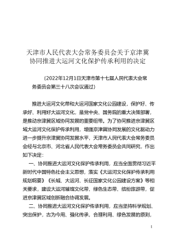
(a) (b) (c) (d)

(e) (f) (g) (h)

Figure 1: Functions in evC(N2,C). The images (a), (d) and (e) are equivalent under warping,

so are (b) and (f), as well as (c), (g) and (h).

Figure 1illustrates eight two-parameter functions (i.e. images), obtained from three

initial functions by repeatedly applying warping.1Hence, the value of any warping

invariant will coincide on pairwise equivalent inputs.

As an example, consider the two-parameter analogon of Equation (1),

Ψr1s:evC(N2,C)→C, X 7→ X1,1−lim

s,t→∞ Xs,t (2)

which is a warping invariant. In fact it belongs to an entire class Ψ of invariants con-

structed as follows.

An N0-valued matrix is called a matrix composition, if it has no zero lines or zero

columns. For every eventually-zero Z∈evC(N2,C), that is lims,t→∞ Zs,t = 0, we deﬁne

the two-parameter sums signature coeﬃcient of Zat the matrix composition avia

⟨SS(Z),a⟩:= X

ι1<···<ιrows(a)

κ1<···<κcols(a)

rows(a)

s=1

cols(a)

t=1

Zas,t

ιs,κt∈C.

Note that this sum over strictly increasing chains ιand κis always ﬁnite since Zis zero

almost everywhere. A numerical illustration is provided in Example 2.6.

We collect the second ingredient for warping invariants. For X∈evC(N2,C) let δX ∈

evC(N2,C) be deﬁned via the forward diﬀerence operator

(δX)i,j := Xi+1,j+1 −Xi+1,j −Xi,j+1 +Xi,j .

1In the sense of Deﬁnition 2.29 each of the eight images is equivalent to one of the initial three.

文档加载中……请稍候！
如果长时间未打开，您也可以点击刷新试试。

下载文档到电脑，查找使用更方便

10 玖币 0人已下载

立即下载

摘要：

Two-parametersumssignaturesandcorrespondingquasisymmetricfunctionsJoschaDiehlLeonardSchmitzUniversityofGreifswaldQuasisymmetricfunctionshaverecentlybeenusedintimeseriesanalysisaspolynomialfeaturesthatareinvariantunder,so-called,dynamictimewarping.Weextendthisnotiontodataindexedbytwoparametersandthus...

展开>> 收起<<

Two-parameter sums signatures and corresponding quasisymmetric functions Joscha Diehl Leonard Schmitz.pdf

共61页,预览5页

还剩页未读，继续阅读

声明：本站为文档C2C交易模式，即用户上传的文档直接被用户下载，本站只是中间服务平台，本站所有文档下载所得的收益归上传人(含作者)所有。玖贝云文库仅提供信息存储空间，仅对用户上传内容的表现方式做保护处理，对上载内容本身不做任何修改或编辑。若文档所含内容侵犯了您的版权或隐私，请立即通知玖贝云文库，我们立即给予删除！

Two-parameter sums signatures and corresponding quasisymmetric functions Joscha Diehl Leonard Schmitz

相关推荐

开通VIP享超值会员特权

作者详情

相关内容

热门标签

举报选择: