
DEEPKOOPMAN LEARNING OF NONLINEAR TIME-VARYING SYSTEMS Wenjian Hao


DEEPKOOPMANLEARNINGOFNONLINEARTIME-VARYINGSYSTEMSWenjianHaoSchoolofAeronauticsandAstronauticsEngineeringPurdueUniversity,IN,USAhao93@purdue.eduBowenHuangPacificNorthwestNationalLaboratoryRichland,USAbowen.h@pnnl.govWeiPanDepartmentofComputerScienceUniversityofManchester,UKwei.pan@tudelft.nlDiWuPacif...
相关推荐
-
岗位管理制度VIP免费
 2024-12-04 20
 -
干部聘任管理制度VIP免费
 2024-12-04 14
 -
法务工作管理制度VIP免费
 2024-12-04 69
 -
发展党员工作制度VIP免费
 2024-12-04 18
 -
对外投资管理制度VIP免费
 2024-12-04 22
 -
独立董事制度VIP免费
 2024-12-04 21
 -
党委会工作制度VIP免费
 2024-12-04 23
 -
安全生产管理制度VIP免费
 2024-12-04 19
 -
“厂务公开、民主监督”制度的实施办法VIP免费
 2024-12-04 22
 -
行政事业单位内部控制报告-关键岗位轮岗及专项审计制度VIP免费

 2025-03-03 318
作者详情

相关内容
-
钢琴谱--勃拉姆斯钢琴谱全集--协奏曲华彩--Cadenza for Beethoven's Piano Concerto in c, Op 37
分类:文学/历史/军事/艺术
时间:2024-12-25
标签:无
格式:PDF
价格:5.9 玖币
-
钢琴谱--勃拉姆斯钢琴谱全集--协奏曲华彩--Cadenza for Bach's Keyboard Concerto in d
分类:文学/历史/军事/艺术
时间:2024-12-25
标签:无
格式:PDF
价格:5.9 玖币
-
钢琴谱--勃拉姆斯钢琴谱全集--协奏曲华彩--2 Cadenzas for Mozart's Piano Concerto in G, K 453
分类:文学/历史/军事/艺术
时间:2024-12-25
标签:无
格式:PDF
价格:5.9 玖币
-
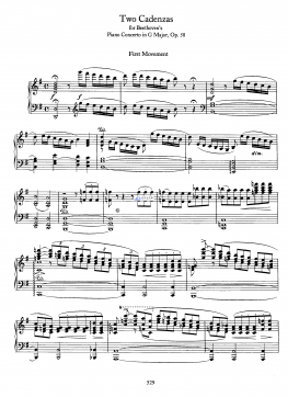
钢琴谱--勃拉姆斯钢琴谱全集--协奏曲华彩--2 Cadenzas for Beethoven's Piano Concerto in G, Op 58
分类:文学/历史/军事/艺术
时间:2024-12-25
标签:无
格式:PDF
价格:5.9 玖币
-
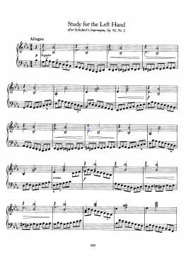
钢琴谱--勃拉姆斯钢琴谱全集--练习曲--Study for Left Hand (after Schubert's Impromptu)
分类:文学/历史/军事/艺术
时间:2024-12-25
标签:无
格式:PDF
价格:5.9 玖币

