
Deep Neural Networks as the Semi-classical Limit of Topological Quantum Neural Networks The problem of generalisation


DeepNeuralNetworksastheSemi-classicalLimitofTopologicalQuantumNeuralNetworks:TheproblemofgeneralisationAntoninoMarcianò,1EmanueleZappala,2TommasoTorda,3MatteoLulli,4StefanoGiagu,3ChrisFields,5DeenChen,6andFilippoFabrocini71CenterforFieldTheoryandParticlePhysics&DepartmentofPhysics,FudanUniversity,Ji...
相关推荐
-
架构演进:小米的经验分享VIP免费

 2025-03-31 26
 -
Chemical Evolution of Fluorine in the Milky Way Kate A. Womack1Fiorenzo Vincenzo1Brad K. Gibson1Benoit Côté23Marco Pignatari3110
 2025-09-29 16
 -
Chemical evolution of elliptical galaxies I supernovae and AGN feedback Marta Molero12Francesca Matteucci123Luca Ciotti4
 2025-09-29 17
 -
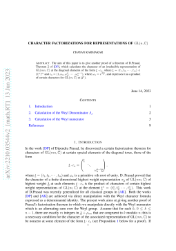
CHAYAN KARMAKAR ABSTRACT . The aim of this paper is to give another proof of a theorem of D .Prasad
 2025-09-29 19
 -
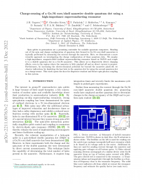
Charge-sensing of a GeSi coreshell nanowire double quantum dot using a high-impedance superconducting resonator
 2025-09-29 17
 -
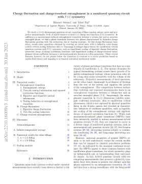
Charge uctuation and charge-resolved entanglement in a monitored quantum circuit with U1symmetry
 2025-09-29 20
 -
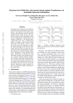
Character-level White-Box Adversarial Attacks against Transformers via Attachable Subwords Substitution
 2025-09-29 21
 -
Certifying randomness in quantum state collapse Liang-Liang Sun1Xingjian Zhang2Xiang-Zhou1Zheng-Da Li34
 2025-09-29 20
 -
CERTIFIED ROBUSTNESS OF QUANTUM CLASSIFIERS AGAINST ADVERSARIAL EXAMPLES THROUGH QUANTUM NOISE
 2025-09-29 19
 -
Certified machine learning Rigorous a posteriori error bounds for PDE defined PINNs
 2025-09-29 20
作者详情
相关内容
-
Charge uctuation and charge-resolved entanglement in a monitored quantum circuit with U1symmetry
分类:图书资源
时间:2025-09-29
标签:无
格式:PDF
价格:10 玖币
-
Character-level White-Box Adversarial Attacks against Transformers via Attachable Subwords Substitution
分类:图书资源
时间:2025-09-29
标签:无
格式:PDF
价格:10 玖币
-
Certifying randomness in quantum state collapse Liang-Liang Sun1Xingjian Zhang2Xiang-Zhou1Zheng-Da Li34
分类:图书资源
时间:2025-09-29
标签:无
格式:PDF
价格:10 玖币
-
CERTIFIED ROBUSTNESS OF QUANTUM CLASSIFIERS AGAINST ADVERSARIAL EXAMPLES THROUGH QUANTUM NOISE
分类:图书资源
时间:2025-09-29
标签:无
格式:PDF
价格:10 玖币
-
Certified machine learning Rigorous a posteriori error bounds for PDE defined PINNs
分类:图书资源
时间:2025-09-29
标签:无
格式:PDF
价格:10 玖币

